GIS Analysis for Typhoon Yagi Relief Efforts in Laos
Sep 25, 2024
Part 1: Population estimates
Background
In early September 2024, Typhoon Yagi devastated parts of Southeast Asia, displacing communities and resulting in significant casualties. Humanitarian organizations required accurate, spatially detailed population data to guide their relief efforts effectively, particularly focusing on vulnerable populations such as children. Makerbox Lao, an organization I co-founded in Laos, was asked if we would be able to contribute data analysis to estimate affected populations using near-live satellite data, helping to direct aid to the most affected regions. Below is the result of this analysis.
The aim was to map age- and sex-stratified population census data to the village level, incorporate population projections to make them up to date, to ensure that UNICEF could target their resources effectively.
Data sources used
- WorldPop Estimates for 2020 (Stratified by Age and Sex)
- Format: Raster
- Provides high-resolution population data, detailing the distribution of different age and sex groups across Laos for the year 2020. We use the top-down dataset, which is a mapping of the district-level census data onto grid estimates of population counts with a grid size of 100×100m. Read about the methods here.
wget -q --recursive --no-parent -nd -P popStructure --accept "lao_m*.tif" "https://data.worldpop.org/GIS/AgeSex_structures/Global_2000_2020/2020/LAO/"
- UNFPA/Lao Statistics Bureau Predictions for Population Growth (2020–2024)
- Format: Tabular data with district-level projections
- Offers projected growth rates for population from 2020 to 2024, per district, allowing for accurate adjustment of population estimates across different regions.
- GADM Dataset for District Boundaries
- Format: Geospatial (vector) data
- Offers district-level administrative boundaries, crucial for aligning population data with administrative regions for consistent analysis and projection. Resolution is available down to level 2, district-level.
- Lao Village Boundaries with District Information
- Format: Geospatial (vector) data
- Contains village-level boundaries and their associated district identifiers, providing granular geographic details necessary for fine-tuning population estimates at a village scale. This provides level 3 polygons, outlining village boundaries. Can be obtained from here.
- Uber H3 Hexagons (Resolution 8)
- Format: Hexagonal grid system
- A spatial indexing system that divides the region into hexagonal cells, enabling standardized aggregation of population data. Resolution 8 hexagons have an average area of around 2.4 km², balancing spatial granularity with manageability.
Objective
With access to flood extents, we can intersect those onto village boundaries, and apply a threshold on the percent of surface covered by floodwater to figure out flood-affected villages. It is then important to be able to figure out these villages’ population by age group. There are no current, granular population estimates in Laos, the last formal census having been run in 2015 and the next one being slated for March 2025. Not only do we need to compute village populations, we also need to adjust them to current predicted levels, which are available at the district level.
Furthermore, for more general affected population estimates, it is useful to have a regular grid on which to estimate population density. We will apply the same masking and adjustment procedure on Uber H3 hexagons.
Analysis workflow
Preprocessing prediction data and mapping it to the village level
Here, just basic data wrangling. We take the village shapefile, read it into a geodataframe, then merge by district ID with the population predictions 2020>2024.
import pandas as pd
# loading in village boundaries
from geopandas import *
lao_adm_boundaries = gpd.read_file('lao_bnd_village_cde2015.shp',  encoding='cp874').to_crs(epsg=4326)

df = pd.read_csv('lao_pop_projections.csv')
# restrict to adm level 2
df = df[df['ADM_LEVEL'] == 2]
# extract columns GEO_MATCH, ADM2_NAME, BTOTL_2020, BTOTL_2024
df = df[['GEO_MATCH', 'ADM2_NAME', 'BTOTL_2020', 'BTOTL_2024']]

# create a new column DCODE in df, by splitting by _, taking the second and third, removing leading zeros, and concatenating without separator
df['DCODE'] = df['GEO_MATCH'].str.split('_').str[1].str.lstrip('0') + df['GEO_MATCH'].str.split('_').str[2]
# convert to integer
df['DCODE'] = df['DCODE'].astype(int)

# merge df with lao_adm_boundaries restricted to columns DCODE, DNAME on DCODE
lao_adm_boundaries_merge = lao_adm_boundaries[['DCODE', 'DNAME']]
# take unique rows
# number of rows before
lao_adm_boundaries_merge = lao_adm_boundaries_merge.drop_duplicates()
print('Number of rows before:', len(lao_adm_boundaries_merge))
df_merged = df.merge(lao_adm_boundaries_merge, on='DCODE', how='left')

# one value has a mistake
# change the value of DCODE in df where DCODE is 1011 to 1013 and redo the merge
df.loc[df['DCODE'] == 1011, 'DCODE'] = 1013
df_merged = df.merge(lao_adm_boundaries_merge, on='DCODE')
Masking WorldPop Data onto Village Geometries
Here, we simply overlay the raster data onto the village polygons, then sum the population values within each polygon to get aggregated estimates stratified by age and sex.
# list all files in the popStructure directory
import os
import rasterio
import numpy as np
from rasterio.mask import mask

filenames = os.listdir('popStructure')

for filename in filenames:
    if filename.endswith('.tif'):
        column_name = os.path.splitext(filename)[0]
        print("Processing", column_name)
        dataset = rasterio.open('popStructure/' + filename)
        print("pop raster CRS:", dataset.crs)

        # Ensure lao_adm_boundaries is in the same CRS as the raster
        lao_adm_boundaries = lao_adm_boundaries.to_crs(dataset.crs)

        lao_adm_boundaries[column_name] = None
        for i, row in lao_adm_boundaries.iterrows():
            geom = [row['geometry']]  # Geometry needs to be in a list
            try:
                out_image, out_transform = mask(dataset, geom, crop=True)
                data = out_image[0]  # Read the first band
                lao_adm_boundaries.at[i, column_name] = np.sum(data[data > -99999])
            except ValueError:
                # Handle cases where the geometry does not intersect the raster
                lao_adm_boundaries.at[i, column_name] = 0
The village geometry file looks like this (classical geoJSON):
After the above operation, we add the following columns:
Index(['lao_f_5_2020', 'lao_f_0_2020', 'lao_f_20_2020', 'lao_m_0_2020',
       'lao_m_40_2020', 'lao_m_10_2020', 'lao_m_55_2020', 'lao_m_70_2020',
       'lao_m_5_2020', 'lao_f_70_2020', 'lao_f_80_2020', 'lao_m_80_2020',
       'lao_f_1_2020', 'lao_f_35_2020', 'lao_m_65_2020', 'lao_m_50_2020',
       'lao_m_30_2020', 'lao_f_25_2020', 'lao_f_60_2020', 'lao_f_15_2020',
       'lao_f_45_2020', 'lao_m_75_2020', 'lao_f_75_2020', 'lao_m_1_2020',
       'lao_f_10_2020', 'lao_m_20_2020', 'lao_f_50_2020', 'lao_m_35_2020',
       'lao_m_45_2020', 'lao_f_55_2020', 'lao_m_25_2020', 'lao_m_60_2020',
       'lao_f_40_2020', 'lao_m_15_2020', 'lao_f_65_2020', 'lao_f_30_2020',
       'geometry'],
      dtype='object')
which represent the stratified populations by sex (_m/f) and age bracket, in 2020.
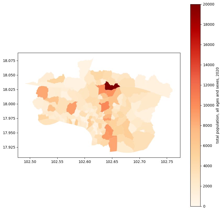
Adjusting village populations based on district-level population estimates
Here, we extract the population estimates per district for 2020 and 2024 in the UNFPA data, calculate the population growth ratio, then merge with the above village dataset by district ID. This allows us to apply scaling to each village based on the district in which they are.
# read in the df_merged which contains the population data
import pandas as pd
df_merged = pd.read_csv('lao_pop_projections_with_DNAME.csv')

# merge both dataframes on DCODE, the pop one subset to BTOTL_2020, BTOTL_2024
gdf=lao_adm_boundaries
merged = gdf.merge(df_merged[['DCODE', 'BTOTL_2020', 'BTOTL_2024']], left_on='DCODE', right_on='DCODE')

# create the ratio of BTOTL_2024 to BTOTL_2020, converting each col to integer and removing commas
merged['ratio'] = merged['BTOTL_2024'].str.replace(',', '').astype(int) / merged['BTOTL_2020'].str.replace(',', '').astype(int)

# for each of the lao_X columns, convert them to numeric, and then multiply by the ratio, creating columns lao_X_2024
for column in merged.columns:
    if column.startswith('lao_'):
        if(merged[column].dtype != 'float64'):
            merged[column] = pd.to_numeric(merged[column], errors='coerce')
        merged[column + '_2024'] = merged[column] * merged['ratio']

# Create 2020 and 2024 columns for the sum of all lao_X columns ending in _2020 and _2024
merged['sum_2020'] = merged.filter(regex='lao_.*_2020$').sum(axis=1)
merged['sum_2024'] = merged.filter(regex='lao_.*_2024$').sum(axis=1)
Using Uber H3 hexagons
We first extract the hexagons that are present within the extent of Laos:
lao_adm_boundaries_union = lao_adm_boundaries[['DCODE', 'TOTAL', 'DNAME','geometry']].dissolve(by='DCODE', aggfunc={'TOTAL':'sum', 'DNAME':'first'})
lao_adm_boundaries_union = lao_adm_boundaries_union.reset_index()

import h3
import geopandas as gpd
from shapely.geometry import Polygon, mapping

# Step 1: Define your bounding box
minx, miny, maxx, maxy = lao_adm_boundaries.total_bounds

# Step 2: Flip coordinates to lat/lon format for h3
bbox_polygon = Polygon([(miny, minx), (miny, maxx), (maxy, maxx), (maxy, minx), (miny, minx)])  # lat/lon format
bbox_geojson = mapping(bbox_polygon)  # Convert to GeoJSON-like structure


# Step 3: Adjust the resolution for larger hexagons initially (e.g., 6)
resolution = 8  # Lower resolution for larger hexagons

# Step 4: Get the list of H3 hexagons that overlap the bounding box
hexagons = h3.polyfill(bbox_geojson, resolution)
Note that it would have been more economical to do a polyfill of the outline of Laos, lao_adm_boundaries_union. I am not sure if that would have worked, but it would have saved time. There are close to a million hexagons over Laos.
# Step 5: Convert H3 hexagons to polygons and store them in a list
hexagon_polygons = []
hex_ids = []
for hex_id in hexagons:
    hex_boundary = h3.h3_to_geo_boundary(hex_id, geo_json=True)
    hexagon_polygons.append(Polygon(hex_boundary))
    hex_ids.append(hex_id)

# Step 6: Create a GeoDataFrame from the list of polygons and hex IDs
hexagons_gdf = gpd.GeoDataFrame({'hex_id': hex_ids, 'geometry': hexagon_polygons}, crs="EPSG:4326")
Now we restrict those to the ones actually overlapping our districts, for each district. If a hexagon maps to >1 district, we get 2 rows per hexagon. We also compute the percentage of the hexagon area in each district:
hexagons_gdf = hexagons_gdf.to_crs(epsg=32648)
lao_adm_boundaries_union = lao_adm_boundaries_union.to_crs(epsg=32648)

# Step 1: Perform a spatial join to find which hexagons intersect with which districts
hex_districts = gpd.sjoin(hexagons_gdf, lao_adm_boundaries_union, how='inner', predicate='intersects')

# Step 2: Merge with the original GeoDataFrame to get the district geometries
hex_districts = hex_districts.merge(lao_adm_boundaries_union[['DCODE', 'geometry']], on='DCODE', suffixes=('', '_district'))

# Step 3: Calculate the intersection area for each hexagon-district pair
hex_districts['intersection_area'] = hex_districts.apply(
    lambda row: row['geometry'].intersection(row['geometry_district']).area,
    axis=1
)

# Step 4: Calculate the fraction of each hexagon within each district
hex_districts['hex_area'] = hex_districts['geometry'].area
hex_districts['fraction'] = hex_districts['intersection_area'] / hex_districts['hex_area']
hex_districts[hex_districts['fraction'] < 0.99].shape[0]/hex_districts.shape[0] gives us 12%, the fraction of polygons that overlap a boundary and belongs to >1 district.
At this point we add the prediction data per hexagon since we already have district information:
# merge hex_districts with df_merged on DCODE
hex_districts = hex_districts.merge(df_merged, on='DCODE')
We mask the population data per hexagon:
import os
import rasterio
import numpy as np
import geopandas as gpd
from rasterio.mask import mask

filenames = os.listdir('popStructure')[1:]

for filename in filenames:
    if filename.endswith('.tif'):
        column_name = os.path.splitext(filename)[0]
        print("Processing", column_name)
        dataset = rasterio.open('popStructure/' + filename)
        print("pop raster CRS:", dataset.crs)
        gdf[column_name] = None
        for i, row in gdf.iterrows():
            geom = [row['geometry']]  # Geometry needs to be in a list
            out_image, out_transform = mask(dataset, geom, crop=True)
            data = out_image[0]  # Read the first band
            gdf.at[i, column_name] = np.sum(data[data > -99999])
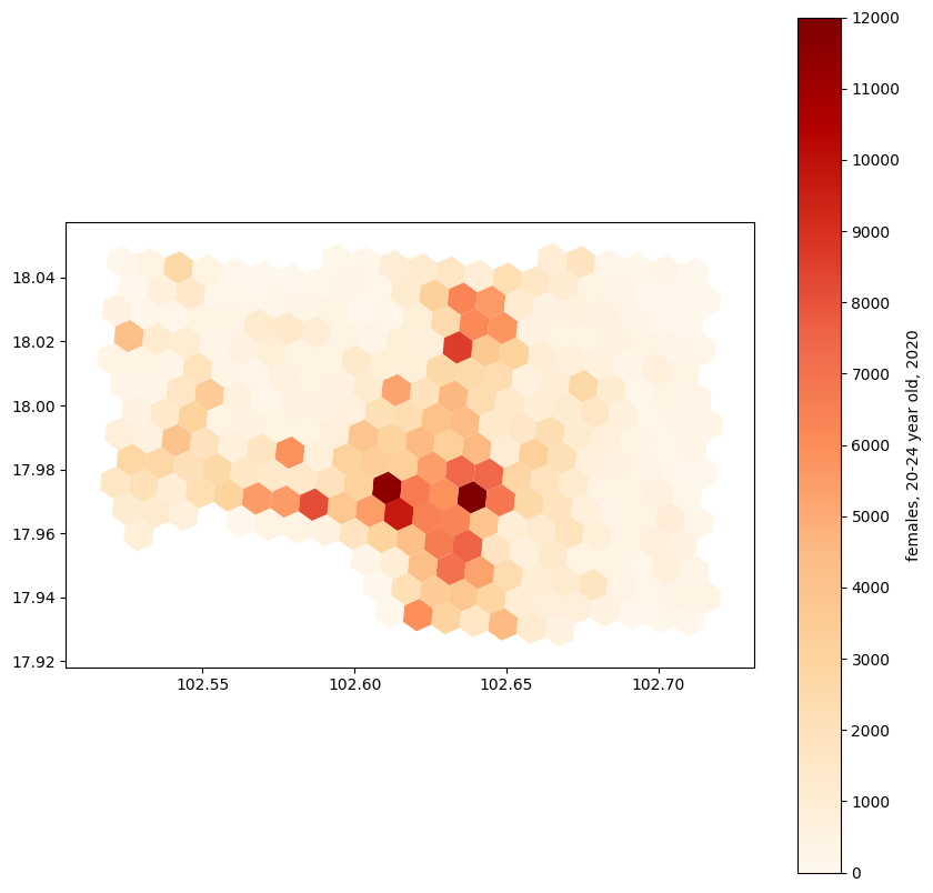
We now need to group by hexagon, and apply scaling per district, then reconstitute single hexagons for the ones that overlap >1 district. This is a costly operation in pandas/python. We use the much faster data.table library in R. This speeds up the analysis by a factor of 10:
import rpy2.robjects as ro
from rpy2.robjects import pandas2ri

# Activate the automatic conversion between pandas and R data frames
pandas2ri.activate()

# subset hexagons df to all columns except geometry
ro.globalenv['mydf'] = hexagons.drop(columns='geometry')
This is a very useful trick allowing us to send data back and forth between the two interpreters in a jupyter notebook running python but with IRkernel installed.
Switching to R:
library(data.table)
mydf=as.data.table(mydf)
proj_columns=grep('_2024',grep('lao_', names(mydf), value=TRUE), value=TRUE)
scaled=mydf[, lapply(.SD, function(x) sum(x*fraction)), by=hex_id, .SDcols=proj_columns]
Now back in python:
scaled=ro.conversion.rpy2py(ro.globalenv['scaled'])
# from hexagons, concatenate DCODE, DNAME_x by hex_id and take the first geometry by hex_id
grouped = hexagons.groupby('hex_id').agg({
    'DCODE': concatenate,
    'DNAME_x': concatenate,
    'geometry': 'first'
}).reset_index()
# merge grouped with scaled on hex_id and rename DNAME_x to DNAME

grouped = grouped.merge(scaled, on='hex_id')
# cast to GeoDataFrame using the same parameters as hexagons
grouped = gpd.GeoDataFrame(grouped, crs=hexagons.crs, geometry='geometry')
Afterword
Feel free to use this code for any similar population analysis or contact me if you need help adapting it. It was certainly enjoyable to go back to GIS analysis in R/Python after a long hiatus. One interesting about GIS is that it often “works”, as in, the analysis completes without errors, but the results may not be what you intended to do. It’s easy to perform masking with bounding boxes instead of geometries, for example, compute areas in geographical (angle-preserving) coordinate systems, or mismatched projections.
This analysis was essentially done as the water was rising, so another challenge was completing it on time and quickly iterating over the better part of a weekend.
In part 2, I’ll go into the other half of this analysis, analysing water level data.
Share