The code for this post is available on GitHub. Any comments are welcome, feel free to raise a GH issue in case of a problem.

Introduction

Copy number variants (CNV) are genetic events in which a portion of the genome gets duplicated or deleted. These events can be relatively innocuous, or have dramatic medical consequences. These events vary greatly in size, from a few kilo-base pairs to entire chromosomes (trisomy 21 is technically a CNV, more specifically a duplication of the whole of chromosome 21).

Most CNV identification tactics are based on whole-genome sequencing, specifically using aligned reads. Moreover, there is no standard file format or generally accepted tool for calling and describing CNVs, despite VCF’s recent efforts to provide a generic file format for storing them. But this state of things means that CNV detection is tricky and resource-intensive, and is mostly restricted to specialised groups who focus on this type of mutation and nothing else. But by and large, a CNV is just another variation, and statistical genetics groups have studied smaller, more traditional variants for ages. In that field, the VCF format is standard, however it only contains information about genetic variation, whereas usual CNV callers need information about the entire genome, more specifically, raw sequencing read data, to call a duplication or deletion event.

So, our question is: can we call copy number variants from single-nucleotide call sets coming from reasonably-covered (>10x) whole-genome sequencing projects? As it turns out, we can.

It’s all about depth

This was a serendipitous discovery. As I was performing quality control for a larger project with Daniel Suveges, we wanted to exclude depth outliers, i.e. samples with not enough, (or too much, but that never happens) sequencing depth. We were doing our measures on chromosome 11 to save time, and were just extracting depth of coverage at every variant using the INFO/DP tag. Based on this, we excluded one individual.

Later, just for peace of mind, I repeated the analysis genome-wide. The outlier disappeared, suggesting that the depth anomaly for that sample was somehow localised to chromosome 11. We plotted the depth for that individual on chromosome 11, and bingo:

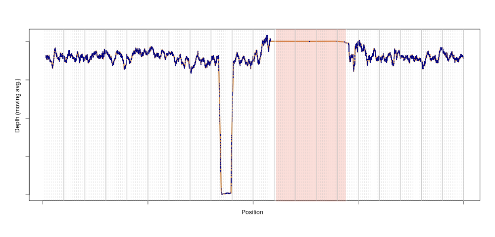
This is exactly what a homozygous deletion could look like: for a stretch of DNA several 100s of kilobase-pairs long, sequencing depth is zero for one sample. That drop in sequencing depth was strong enough to make the sample an outlier for depth on this entire chromosome (the shaded region is the centromere, where no variants are present). Of course, as soon as we knew there could be something in that region, we looked across the entire population, and again, a clear pattern emerged:

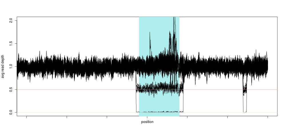
Not only did we see a clear concentration around 0.5 and 0 relative depth for that particular region, we saw that there was likely another deletion event close-by, too small to have a large impact on the depth, so too small for us to notice using the method above. This was also very encouraging, because we were likely not seeing sequencing artifacts, as hard-to sequence regions have no reason to be exactly half as hard to sequence (yielding 0.5 relative depth), and so the method was born.

I guess our main surprise was that the signal was so clean. Looking at the depth distribution around that region was almost too good to be true, with very clear boundaries around \(\LARGE0.5\pm.05\) relative depth.

Automating detection of boundaries with a regression tree

So, as an applied mathematician (if there is such a thing), I immediately thought “we need to fit a piecewise constant function to this”. Which means, basically, that we would fit a very constrained model that only allows for our depth to be constant along a certain stretch of DNA, then drop to 0 (or 0.5 for heterozygotes), then back to a constant 1 again. In machine learning lingo, this method is called a regression tree. So, we use the very nifty and easy to use rpart R method to fit such a tree to the raw depth measures for our homozygous sample:

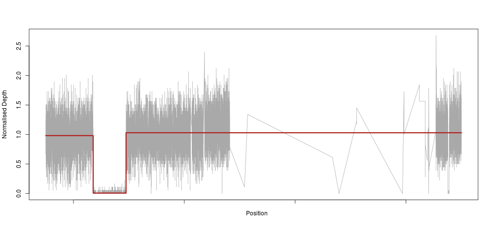
The model reacts perfectly (note the very sparse centromeric region again) with a clear drop to zero in the region of our deletion. This is essentially an extreme downsampling of the frequency of our depth signal.

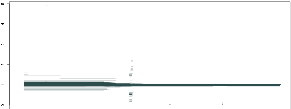
So, what happens if we do this not just for 1 individual, but across a population of about ~1300 samples, and plot all piecewise constant fragments together? A thing of beauty:

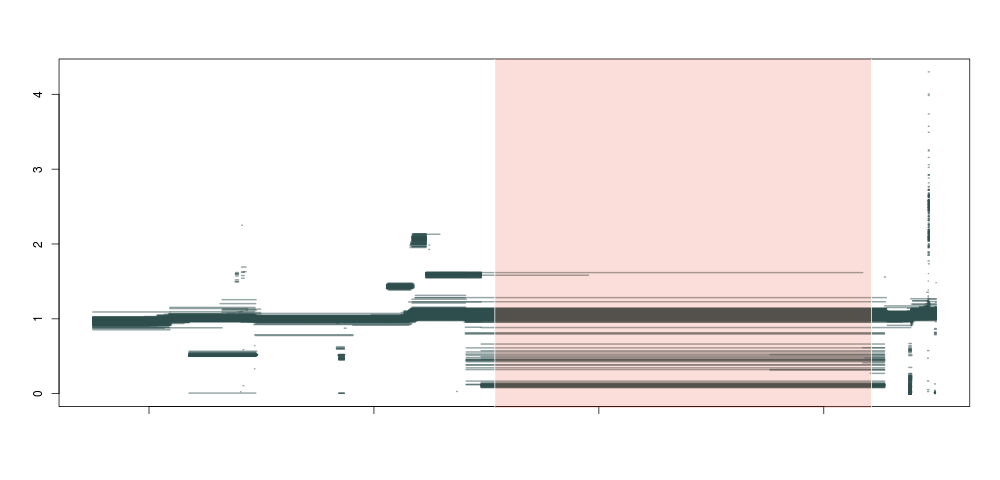
Producing this is as simple as running the code below for each sample:

regiondata=data.frame(pos=dfcall$pos, dp=dfcall[,selected_sample]/chrwide_depth[selected_sample])
tree <- rpart(dp ~ pos, data=regiondata)
x=regiondata$pos
s <- seq(min(x), max(x), by=100)
pred=predict(tree, data.frame(pos=s))
downsampled=data.frame(pos=seq(min(x), max(x), by=100), pred=pred)
ret=cbind(aggregate(downsampled$pos, by=list(downsampled$pred), min), aggregate(downsampled$pos, by=list(downsampled$pred), max)$x)
colnames(ret)=c("depth", "min","max")
ret$sample=selected_sample

Here we see that not only are our deletion boundaries clearly delineated, there are much more complex events happening within it (small duplications or repeats), and we can also clearly see duplications (clusters around 1.5 and 2 between our deletion and the centromere) and hard-to-map regions (the vertical bar towards the right end of the plot) probably composed of repeats. We have effectively transformed the depth signal from our VCF single-nucleotide calls into an exhaustive description of depth anomalies genome-wide. And extracting the relevant info was extremely simple. As in:

bcftools query -f '%CHROM\t%POS\t[%DP\t]\n' file.vcf.gz

Looking at the distribution of our constant fragments, we again notice clear peaks around the expected heterozygous and homozygous deletion and duplications:

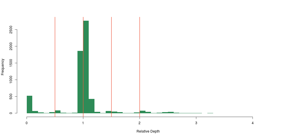
A first, crude deletion caller

Clearly, to call boundaries we need to aggregate these breakpoints, and add our prior knowledge about where “real” breaks will occur. For deletions, as we have said, we expect \(\LARGE\{0,0.5,1\}\).

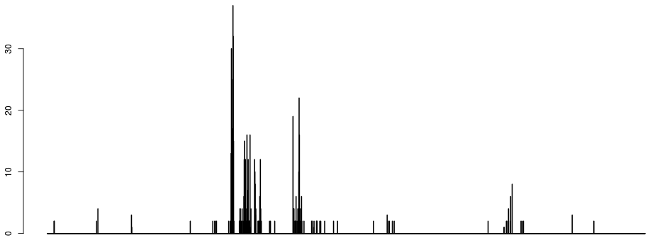
If we discretize the x axis and plot the number of breakpoints occurring per bin, we get something like:

Two things to note here:

• just counting breakpoints is unsatisfactory, as most breaks occur around 1. The next strongest signal is around the hard-to-map region right of the centromere, which is logical given the large depth heterogenity in that region. The signal that we want to see (the two dots around 0 to the right) is very weak on the histogram of breaks.
• the first parameter of the algorithm is emerging: namely the discretisation of the x axis. This parameter does not have a huge influence, apart from the fact that CNVs smaller than the discretisation window are at risk of being incorrectly called.

To address the first point, we only count breakpoints occurring around narrow bands around 0.5 and 0:

# alldepth is a dataframe containing the columns min, max, depth for each sample and each constant depth fragment 
discr=seq(min(allbreaks$min), max(allbreaks$max), by=5000)
numhethom=sapply(discr, function(x){
    a=alldepth[allbreaks$min<=x & allbreaks$max>=x,];
    b=table(cut(a$depth, breaks=c(0,5*mad(allbreaks$depth), 0.5-5*mad(allbreaks$depth), 0.5+5*mad(allbreaks$depth), max(allbreaks$depth))))
    return(b[1]+b[3])
    })

The boundary we choose here is \(\LARGE 5\times MAD\left(depth_{segments}\right)\), the MAD being the median absolute deviation. This is again a rather arbitrary threshold, and the code above handles only deletions. More on that later.

The above gives us the number of breakpoints we are interested in across a discretisation of the x axis. To extract the boundaries of the structural variants we must take into account the fact that boundaries might not be exactly the same for two samples. We make use of the very elegant rle R function, which gives us the runs of equal values in a vector. If we do a rle(numhethom>0) we will be extremely sensitive: we will call a CNV wherever there is a breakpoint in the regions around 0 or 0.5. We define a rather arbitrary threshold limit_detection=floor(mean(numhethom)/16) equal to \(\LARGE\frac{1}{16}^{th}\) of the expected number of such breakpoints to circumvent that problem.

limit_detection=floor(mean(numhethom)/16)
a=rle(numhethom>limit_detection) 
svs=t(rbind(a$values, a$lengths, min(discr)+cumsum(a$lengths)*5000))
svs=svs[svs[,1]==1,]
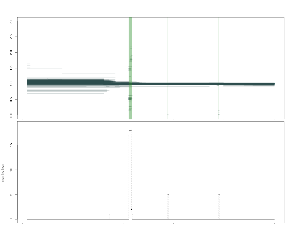
rect(xleft=svs[,3]-svs[,2]*5000, xright=svs[,3], ybottom=-1e6, ytop=1e6, border=NA, col=adjustcolor("forestgreen", alpha=0.4))
plot(discr, numhethom,type="l", lty=2, col="gray")
points(discr, numhethom, pch=".", cex=2)

This gives a very satisfying result:

A subtler caller

Although this first attempt gives some nice results, we would like to do away with several of its limitations, notably the arbitrary thresholds used to determine when to call a variant.

To do this, we can use the fact that we know precisely what the depths should be for a hom/het deletion. We can also hypothesize that if we had an unlimited sample size, we would see the same distribution of segments around 0 and 0.5 as we see now around 1.

This corresponds to a Gaussian mixture model with \(\LARGE k\) the number of normal distributions equal to the number of multiples of 0.5 at which a depth segment is observed, like so:

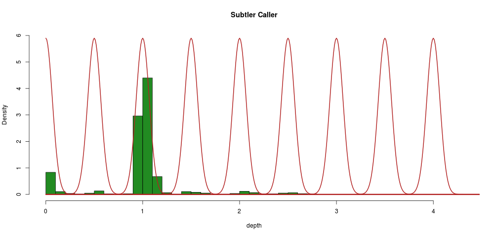
We can constrain the algorithm in the following ways:

• means should be equal to multiples of 0.5
• standard deviations should be equal as per the hypothesis above

Practically what we will do is to build a distribution around 1 (where we have loads of data), and then shift that by multiples of 0.5. The major advantage of this method is that it gives us a probability of every segment (sample) belonging to a given distribution, i.e., we have a probability attached to every call.

Practically, we implement this in R using the very convenient normalmixEM function, part of the mixtools package:

## allbreaks is a data frame like the 'ret' one above
library(mixtools)
mvect=seq(0, ceiling(max(allbreaks$depth)), by=0.5)
mix=normalmixEM(allbreaks$depth, k=length(mvect), mu=mvect, sigma=1, mean.constr=mvect, sd.constr=rep('a', length(mvect)))
parm=cbind(mix$mu, mix$sigma)

This allows us to call an “assigned depth” for every segment and give it a probability:

callz=t(sapply(allbreaks$depth, function(meas) {
    botparm=parm[parm[,1]==floor(meas*2)/2,]
    topparm=parm[parm[,1]==ceiling(meas*2)/2,]
    topp=max(pnorm(meas, mean=botparm[1], sd=botparm[2], lower.tail=F), pnorm(meas, topparm[1], sd=topparm[2], lower.tail=T))
    topn=ifelse(pnorm(meas, mean=botparm[1], sd=botparm[2], lower.tail=F)>pnorm(meas, topparm[1], sd=topparm[2], lower.tail=T), botparm[1], topparm[1])
    return(c(meas, 2*topp, topn))
}))
allbreaks$assigned_depth=callz[,3]
allbreaks$p_value=callz[,2]

Then we set a confidence (minimum p-value to consider inclusion in a given assigned depth), then build 2 different indicators that will tell us at each position:

1. how many segments are above confidence
2. the ratio of high/low confidence segments

confidence=0.05 # we are being lenient, about +/-3SD
tocall=allbreaks[allbreaks$assigned_depth<1, ] # replace this with != to call dups and dels
discr=seq(min(alldepth$min), max(alldepth$max), by=5000)

numhethom=sapply(discr, function(x){
    in_region=tocall[tocall$min<=x & tocall$max>=x,]
    nrow(in_region[in_region$p_value>confidence,])
    })
numhethom2=sapply(discr, function(x){
    in_region=tocall[tocall$min<=x & tocall$max>=x,]
    if(nrow(in_region)==0){return(0)}
    adjust_factor=nrow(in_region[in_region$p_value<confidence,])
    if(!is.finite(adjust_factor)){adjust_factor=1}
    nrow(in_region[in_region$p_value>confidence,])/adjust_factor
    })

Then we can use our rle function again to call a variation when either numhethom or numhethom2 pass a certain threshold.

The current version of the caller is very permissive: it uses numhethom, so the number of high-confidence segments, and has a threshold of 0. Any region that has at least one high-confidence call will be named a CNV. This allows extreme sensitivity (you can call singletons) but it will fail to filter out hard to map regions (where numhethom2 would be much lower).

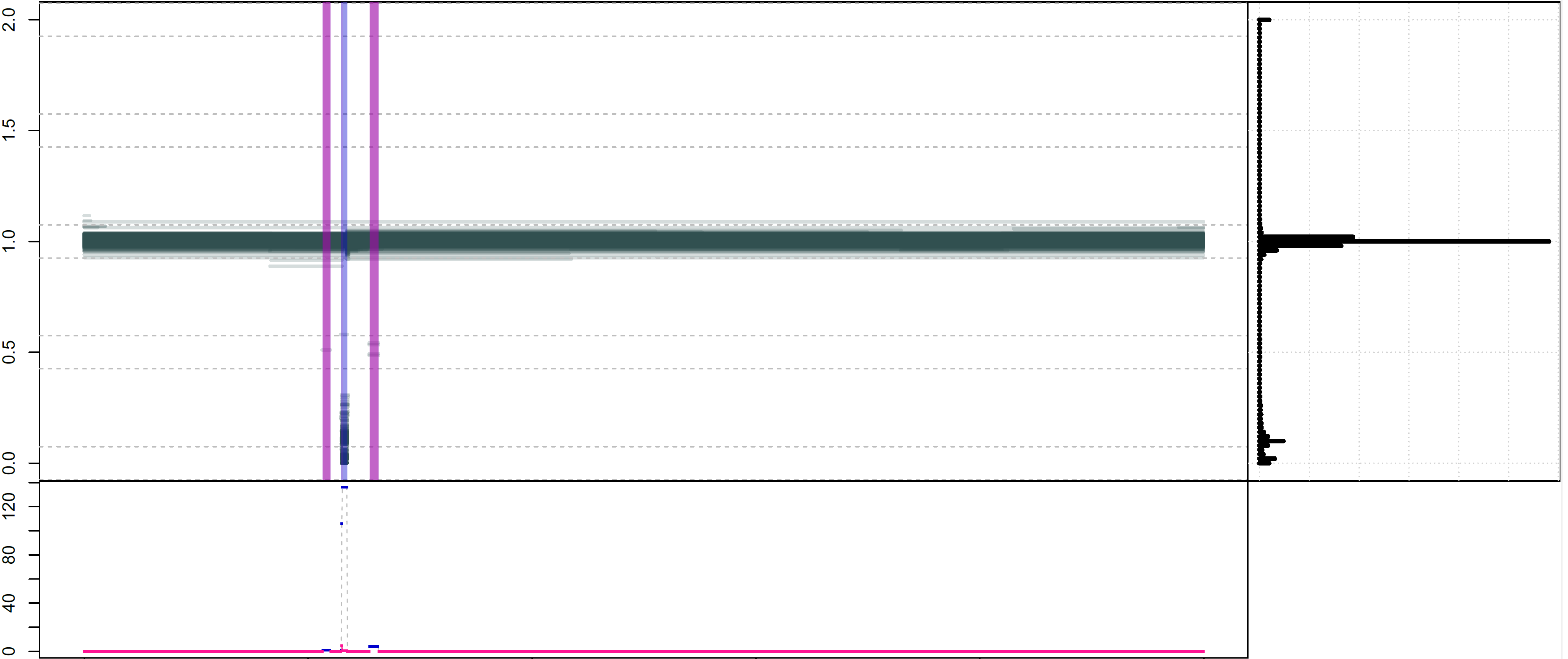
This is illustrated in the image below, where the purple regions are called as variant by both metrics, and the blue one only by the more permissive numhethom. Clearly, the one in blue is of lower quality, with a lot of segments of intermediate depth that are less likely to correspond to a real deletion. Both statistics are represented below the plot, as expected the blue numhethom is much higher than the red numhethom2 over the contentious region.

In practice, I would recommend to either:

• run the caller as is (very sensitive), and use the diagnostics file that is produced with every call to filter out the calls you don’t like;
• or use numhethom2 and adjust the threshold for it in the rle call. It is probably a good idea to use a threshold similar to what we did above, something locally defined like mean(numhethom2)/l where \(\LARGE l \lt 1\) is an arbitrary multiplier of your choice.

The code is on GitHub and is pretty minimal, but enough to start playing around and convert your SNP data to CNVs. As usual I’m available for any questions.

Happy calling!