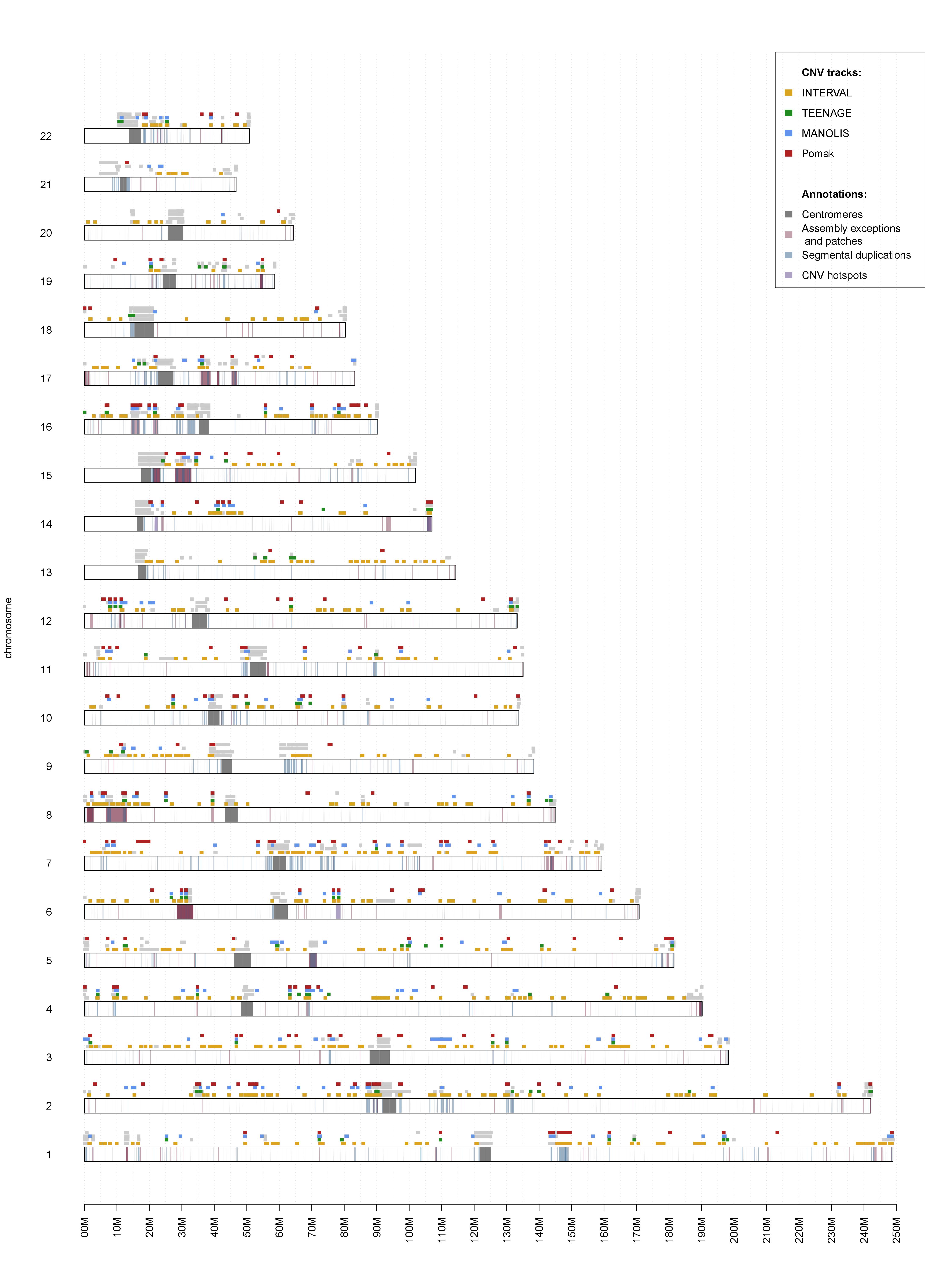
A while ago I set aside a few weekends to play around with VCF files. I wanted to see if depth information at marker sites was enough to reliably call large CNVs in population-scale WGS studies. As it turned out, it was not only possible but very efficient compared to read-based methods. The rudimentary caller I wrote has matured into a useable program called UN-CNVc, which has been used to describe four European populations comprising over 6,000 samples. This side project has now materialised into a full-fledged article, which can be viewed on BioRxiv. One of the most impressive outputs (in my opinion) is this cross-population CNV map:

Summary of the method

Below are some of the main characteristics of UN-CNVc that differentiate it from other algorithms:

• the only input required is a VCF file. Currently, the program uses per-chromosome files, but it can be easily modified for genome-wide VCFs;
• UN-CNVc does not normalise according to GC content, because in cases we examined, GC variations have a much higher frequency than the lower detection limit of UN-CNVc. It is, however, very easy to add a GC-correction step in the code, prior to calling.
• The caller performs per-sample piecewise constant regression and aggregates the resulting depth segments over all samples. Although the approach can be used for a single sample, population scale datasets give context and allow to differentiate between high and low-quality calls. We recommend to run UN-CNVc on samples greater than 100 individuals.
• The algorithm needs to be able to make a difference between relative depths of 0.5. This is relatively small, especially when accounting for the usually large depth variations around the ideal depth. This means that a high average depth will dramatically increase the precision of the caller. We tested the software with depths ranging from 18 to 40x. We recommend depths greater than 15x.
• The program’s resolution is limited by the average distance between two SNPs and the discretisation step. For studies composed of a few thousands samples, we found this was equivalent to a resolution of roughly 5~10kb. But interestingly, this particularity means UN-CNVc’s precision should improve as sample sizes increase.

Discussion on the Gaussian model

Currently, segment depth is modelled as a mixture of Gaussians with equal variances and means constrained to multiples of 0.5 relative depths. However, the Poisson model of read depth yields that variances should be proportional to the mean. Another commonly used model for read depth is the negative binomial, which deals with overdispersion at high depths (as depth increases, the variance increases more than can be expected under the Poisson model).

We found that the Gaussian model performed adequately in our settings, but this overdispersion means that UN-CNVc likely underestimates the variance at high copy numbers, which in turn underestimates the quality of copy number calls. Conversely, at depths below 1, overestimating the variance may produce overconfidence in deletion calls.

I am not fully convinced by the Poisson and NB models in this setting, however, mainly because of what happens at depth 0. The expected read depth is null, and therefore the variance is null as well. This means that the model distribution is a Dirac impulsion at 0, which is clearly not suitable for any kind of real-world modelling. So I would likely need to tweak the distribution model to allow non-null variance at zero, given that zero calls are arguably the most interesting (homozygous deletions).

There is another argument in favour of choosing a Gaussian model.

A scaled Poisson distribution, while obviously not Poisson-distributed, follows a Poisson-like distribution with a PDF of \(\Large p(x)=e^{-\lambda}\frac{\lambda^{\frac{x}{c}}}{ \frac{x}{c} !}\). A sum of independent Poisson variables \(\Large X_1,…,X_n\) with parameters \(\Large\lambda_1,…,\lambda_n\) is Poisson distributed with parameter \(\Large\sum_n{\lambda_i}\). The average of these variables follows the scaled Poisson described above, where \(\Large c=\frac{1}{n}\). Poisson distributions can be approximated by the normal when \(\Large\lambda\) is very large. Although the normal approximation is likely invalid for any of the \(\Large X_1,…,X_n\) at usual WGS depths such as the 22x average in MANOLIS, the sum or average, with a parameter \(\Large\sum_n{\lambda_i}\), is closer to the normal approximation.

This leads me to think that the next step in UN-CNVC’s development may indeed be to tweak the depth model, but not to replace it with a Poisson or NB model. Instead, it would probably be sensible to release the equality of variance constraint, and model each component of the mixture separately. A genome-wide estimation would compensate the local paucity of anomalous depth segments, although it would also slow the program down.

As often when writing bioinformatics tools, design choices have opposing impacts on execution speed and accuracy.